14.5 Some notes about Just-Dice.com gambling probabilities part 3

3rd August, 2013

Other posts in series

Suggested reading:

14.2 Some notes about Just-Dice.com gambling probabilities part 1

14.4 Some notes about Just-Dice.com gambling probabilities part 2

0. Introduction

In a discussion with bitcointalk.org forum member Dabs, I realised that trying to publish short posts to explain gambling probability was working against many readers completely understanding them. If there's anything you don't understand, please post a comment - if you don't understand then I haven't done what I've set out to do.

The discussion with Dabs has lead me to change nomenclature slightly which the example below (from the aforementioned discussion) will explain.

Consider the following 21 on 50% to win just-dice.com, calling "loss" = 0 and "win" = 1:

0 0 0 1 0 1 0 0 1 1 1 0 0 0 0 0 0 1 1 0 1

Now split into the "roll number", "run (or sequence) number" and "losses per run":

Rolls: 0  0  0  1    0  1    0  0  1    1    1    0  0  0  0  0  0  1    1    0  1

Roll

number: 1  2  3  4    5  6    7  8  9    10   11   12 13 14 15 16 17 18   19   20 21

Run

number: 1             2       3          4    5    6                      7    8

Losses

per run:3             1       2          0    0    6                      0    1

I hope the above makes the concepts of "loss runs" and "losses per run" simpler for readers. Also, since "Run number" and "Number of wins" are different ways of referring to the same random variable, I'll be using the term "wins" instead of "loss runs" from now on.

1 Median number of wins m before more than n losses in a row

In the last post I derived a formula to allow you to calculate the expected (or average) number of wins before more than n losses in a row:

The median number of wins before more than n losses in a row is that random variable that has a cumulative probability of 50% of occurring, ie for a given random variable Y, Pr(Y > m) = 0.5 if m is the median random variable. Knowing this allows a calculation of the median number of wins before n losses in a row.

In the derivation which follows, X is the "losses in a row before a win" random variables,  Y is the "number of wins until n losses in a run" random variables, pX is the probability of variable X occurring, and pY the probability of Y occurring.

Recall that the second CDF function is different from the first since this is a "shifted" geometric distribution. While the number of loss before a win can be 0, 1, 2, 3 ..., the number of wins can only be 1, 2, 3, 4, ....

The lower truncated square brackets denote the "ceiling" operator. It simply means to "round up" the  enclosed formula. This is because a discrete random variable must be an integer, so the median must be an integer too, and the result must be rounded up since the number of wins cannot be less than 1.

The chart below shows the change in mean and median wins for the number of losses before a win for a 50% chance to win game.

2 Any percentile of wins before more than n losses in a row

 The median random variable is that which equates to a lower tail probability of 0.5 - that is 50% of all variables in a sample will be smaller than or equal to this variable. Other probabilities give result in different variables. For example, the 99th percentile variable arises from a lower tail probability of 0.99 and 99% of a sample will be smaller than this variable.

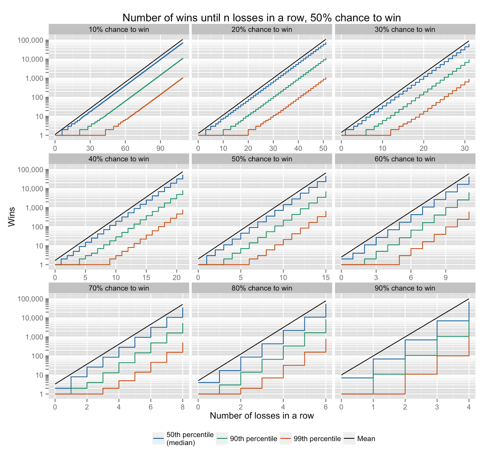
If you're planning how much bank you need in order to outlast n losses in a row, you will probably want to use a guide that will be accurate 90% or 99% of the time, rather than 50% of the time. The median number of wins before n losses in a row will occur 50% of the time - but the 90% or 99% percentile number of wins before n losses in a row will be exceeded only 10 or 1 % of the time.

The chart below shows the mean, median, 90th and 99th percentile wins for the number of losses before a win, for a 50% chance to win game, on a log - linear scale.

So, for example although 6 losses in a row will be expected to occur at 128 wins, it will also occur after 89 wins 50% of the time, after 14 wins 90% of the time, and after 2 wins 99% of the time. For the last two this also means that 6 losses in a row will occur before or at 14 wins 10% of the time and before or at 2 wins 1% of the time.  Depending on your tolerance for risk, you can choose to avoid 6 losses in a row any arbitrary percentage of the time.

Same chart, but for various probability games:

Data in csv format:
10% chance to win

20% chance to win
30% chance to win
40% chance to win
50% chance to win
60% chance to win
70% chance to win
80% chance to win
90% chance to win

3. Summary

So you're probably wondering "How can I use this to help me bet?". Well, it can help you bet safely. If you can budget to withstand a certain number of losses in a row, then you can work out how likely they are to occur before an arbitrary number of wins. The higher the confidence probability you set, the safer you will be.

In the formula below, choose a confidence probability pC (I recommend 0.8 to 0.99, the closer to 1 the safer you'll be) for a game with a probability to win of pX to calculate the number of wins before n losses in a row with confidence pC.

For those wanting to copypaste into a spreadsheet of some sort, try the formula below, although I don't know what the Excel version of the "ceiling" function is:

ceiling(ln(pC)/ln(1 - (1 - pX)^(n + 1))

If you don't want to do that, you can also use the tables from the last section.

Good luck!

organofcorti.blogspot.com is a reader supported blog

BTC:  12QxPHEuxDrs7mCyGSx1iVSozTwtquDB3r

For notification of new posts, follow @oocBlog

Math published using QuickLaTeX and codecogs.

<fourteenpoint five>